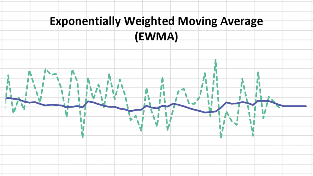
Exponentially Weighted Moving Average (EWMA)
After receiving several inquiries about the exponentially weighted moving average (EWMA) function in NumXL, we decided to dedicate this issue to exploring this simple function in greater depth.
The main objective of EWMA is to estimate the next-day (or period) volatility of a time series and closely track the volatility as it changes.
Background
Suppose the value of the market variable at the end of day $i$ is ${{S}_{i}}$. The continuously compounded rate of return during day I (between end of prior day (i.e. $i-1$) and end of day $i$) is expressed as:
${{r}_{i}}=\ln \frac{{{S}_{i}}}{{{S}_{i-1}}}$
Next, using the standard approach to estimate ${{\sigma }_{n}}$ from historical data, we’ll use the most recent m-observations to compute an unbiased estimator of the variance:
$\sigma _{n}^{2}=\frac{\sum\limits_{i=1}^{m}{{{({{r}_{n-i}}-\bar{r})}^{2}}}}{m-1}
$
Where $\bar{r}$ is the mean of ${{r}_{i}}$:
$\bar{r}=\frac{\sum\limits_{i=1}^{m}{{{r}_{n-i}}}}{m}$
Next, let’s assume $\bar{r}=0 $ and use the maximum likelihood estimate of the variance rate:
$\sigma _{n}^{2}=\frac{\sum\limits_{i=1}^{m}{r_{n-i}^{2}}}{m}$
So far, we have applied equal weights to all $r_{n}^{2}$ , so the definition above is often referred to as the equally-weighted volatility estimate.
Earlier, we stated our objective was to estimate the current level of volatility ${{\sigma }_{n}}$, so it makes sense to give higher weights to recent data than to older ones. To do so, let’s express the weighted variance estimate as follows:
$\sigma_n^2=\sum_{i=1}^m \alpha_i \times r_{n-i}^2$
Where :
- ${{\alpha }_{i}}$ is the amount of weight given to an observation i-days ago.
- ${{\alpha }_{i}}\ge 0$
- $\sum\limits_{i=1}^{m}{{{\alpha }_{i}}}=1$
So, to give higher weight to recent observations, ${{\alpha }_{i}}\ge {{\alpha }_{i+1}}$.
Long-run Average variance
A possible extension of the idea above is to assume there is a long-run average variance ${{V}_{L}}$ , and that it should be given some weight:
$\sigma_n^2=\gamma V_L+\sum_{i=1}^m \alpha_i \times r_{n-i}^2$
Where:
- $\gamma +\sum\limits_{i=1}^{m}{{{\alpha }_{i}}}=1$
- ${{V}_{L}}>0$
The model above is known as the ARCH (m) model, proposed by Engle in 1994.
$\sigma _{n}^{2}=\omega +\sum\limits_{i=1}^{m}{{{\alpha }_{i}}r_{n-i}^{2}}$
EWMA
EWMA is a special case of the equation above. In this case, we make it so that the weights of variable ${{\alpha }_{i}}$ decrease exponentially as we move back through time.
${{\alpha }_{i+1}}=\lambda {{\alpha }_{i}}={{\lambda }^{2}}{{\alpha }_{i-1}}=….={{\lambda }^{n+1}}{{\alpha }_{i-n}}$
Unlike the earlier presentation, the EWMA includes all prior observations, but with exponentially declining weights throughout time.
Next, we apply the sum of weights such that they equal the unity constraint:
$\sum\limits_{i=1}^{\infty }{{{\alpha }_{i}}={{\alpha }_{1}}}\sum\limits_{i=0}^{\infty }{{{\lambda }^{i}}=}1$
For $\left\| \lambda \right\|<1 , \text{the value of }{{\alpha}_{1}}=1-\lambda $
Now we plug those terms back into the equation. For the $\sigma _{n-1}^{2}$ estimate:
$\begin{align}& \sigma _{n-1}^{2}=\sum\limits_{i=1}^{n-1}{{{\alpha }_{i}}}r_{n-1-i}^{2}={{\alpha }_{1}}r_{n-2}^{2}+\lambda {{\alpha }_{1}}r_{n-3}^{2}+…+{{\lambda }^{n-3}}{{\alpha }_{1}}r_{1}^{2} \\ & \sigma _{n-1}^{2}=(1-\lambda )(r_{n-2}^{2}+\lambda r_{n-3}^{2}+…+{{\lambda }^{n-3}}r_{1}^{2}) \\
\end{align}$
And the $\sigma _{n}^{2}$ estimate can be expressed as follows :
$\begin{align}
& \sigma _{n}^{2}=(1-\lambda )(r_{n-1}^{2}+\lambda r_{n-2}^{2}+…+{{\lambda }^{n-2}}r_{1}^{2}) \\
& \sigma _{n}^{2}=(1-\lambda )r_{n-1}^{2}+\lambda (1-\lambda )(r_{n-2}^{2}+\lambda r_{n-3}^{2}+…+{{\lambda }^{n-3}}r_{1}^{2}) \\
& \sigma _{n}^{2}=(1-\lambda )r_{n-1}^{2}+\lambda \sigma _{n-1}^{2} \\
\end{align}$
Now, to understand the equation better:
$\begin{align} & \sigma _{n}^{2}=(1-\lambda )r_{n-1}^{2}+\lambda \sigma _{n-1}^{2} \\ & \sigma _{n}^{2}=(1-\lambda )r_{n-1}^{2}+\lambda ((1-\lambda )r_{n-2}^{2}+\lambda \sigma _{n-2}^{2}) \\ \end{align}$
$\cdots$
$\sigma_n^2=(1-\lambda)(r_{n-1}^2+\lambda r_{n-2}^2+\lambda^2 r_{n-3}^2+\cdots+\lambda^{k+1} r_{n-k}^2)+\lambda^{k+2}\sigma_{n-k} \\$
For a larger data set, the ${{\lambda }^{m+2}}\sigma _{n-m}^{2}$ is sufficiently small to be ignored from the equation.
The EWMA approach has one attractive feature: it requires relatively little stored data. To update our estimate at any point, we only need a prior estimate of the variance rate and the most recent observation value.
A secondary objective of EWMA is to track changes in the volatility. For small $\lambda $ values, recent observations affect the estimate promptly. For $\lambda $ values closer to one, the estimate changes slowly based on recent changes in the returns of the underlying variable.
The RiskMetrics database (produced by JP Morgan and made public available) uses the EWMA with $\lambda =0.94$ for updating daily volatility.
Lambda ($\lambda$)
A secondary objective of EWMA is to track changes in the volatility, so for small $\lambda $ values, recent observation affect the estimate promptly, and for $\lambda $ values closer to one, the estimate changes slowly to recent changes in the returns of the underlying variable.
The RiskMetrics database (produced by JP Morgan) and made public available in 1994, uses the EWMA model with $\lambda =0.94$ for updating daily volatility estimate. The company found that across a range of market variables, this value of $\lambda $ gives forecast of the variance that come closest to realized variance rate. The realized variance rates on a particular day was calculated as an equally-weighted average of $r_{i}^{2}$ on the subsequent 25 days.
$\sigma _{n}^{2}=\frac{\sum\limits_{i=0}^{24}{r_{n+i}^{2}}}{25}$
Similarly, to compute the optimal value of lambda for our data set, we need to calculate the realized volatility at each point. There are several methods, so pick one. Next, calculate the sum of squared errors (SSE) between EWMA estimate and realized volatility. Finally, minimize the SSE by varying the lambda value.
Sounds simple? It is. The biggest challenge is to agree on an algorithm to compute realized volatility. For instance, the folks at RiskMetrics chose the subsequent 25-day to compute realized variance rate. In your case, you may choose an algorithm that utilizes Daily Volume, HI/LO and/or OPEN-CLOSE prices.


