Handling Missing Values
This issue is the first in a series of articles that explore the data preparation aspect of time series analysis. Data preparation is often overlooked by analysts, but we believe it is a vital phase that wields a vast influence on the overall analysis and modeling process. The vast majority of time series and econometric theories assume input time series to be stationary and homogenous, with equally-spaced observations and values that are present and real. In practice, we often handle samples with missing values, unequally-spaced observations possible outliers, mean/variance dependency, restricted values ranges, and other phenomena. The aim of this series of articles is to address each of these problems and introduce practical methods to overcome them.
In this issue, we start with the sampling assumptions of the time series: equal spacing and completeness. Then we consider a time series with missing values and discuss how to represent them in Excel, with the aid of NumXL processing. Finally, we look at unequally-spaced time series, how they come into existence, how they are related to the missing values scenario, and what to do with them.
Time-Series Sampling
The common (perfect) situation for a time series sample is one that has equally-spaced observations and present values for all points. This arises either because observations are made deliberately at even intervals (continuous process), or because the process only generates outputs at such an interval in time (discrete process).
Furthermore, the time-unit for a sampling period (i.e. step) between two consecutive observations can be either absolute (e.g. daily, weekly, monthly, or annual), or based on a holiday calendar (i.e. adjusted for weekends and holidays). For example, a daily financial time series of IBM stock closing prices are based on the NYSE holidays calendar, so each observation is taken on an NYSE trading day (open/close).
With respect to time series modeling and forecasting, it is not important whether we use absolute time or if we adjust for weekends and holidays. What is important is how we interpret the out-of-sample dates, as they too are based on the same sampling method.
Next, let’s examine some cases where the input time series is not so perfect.
Issue 1: Missing Values
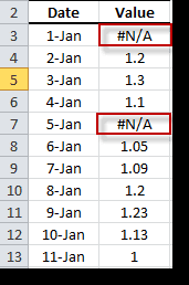
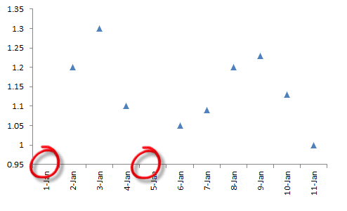
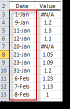
In some situations, one or more observation dates yield invalid or missing values. These values are designated as “Not a Number values” or NaN for short. In Excel, NaN is identified by the special “#N/A” representation, and few built-in functions can be used to detect (e.g. NA (), ISNA (.), IFERROR (.), etc.) or ignore them (e.g. MIN (.), MAX (.)), and other functions are not supported.
In time series analysis, we often encounter missing values phenomena, either in the original raw time series or as a result of a time series operator (e.g. lag, differencing, etc.).
NumXL has two simple rules:
- The missing values at the beginning or at the end of the time series are simply ignored. NumXL will truncate the input time series to start from the 1st non-missing value and end with the last non-missing value.
- The intermediate missing values are considered serious flaws in the input time series, and NumXL can’t process them.
These rules beg the question: how do we handle missing intermediate values?
Many techniques have been proposed to handle time series with missing data, but we can summarize these proposals with two principles: ignore and interpolate.
IGNORE
The ignore solution simply drops the missing value from the time series. You can use the NumXL RMNA (.) function for this purpose. However, you should approach this solution cautiously as it alters the sampling of the time series itself.
INTERPOLATE
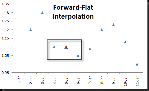
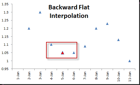
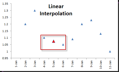
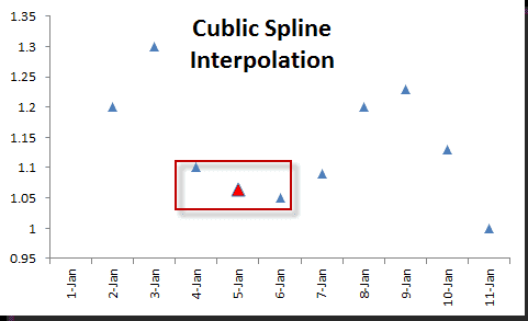
The interpolate approach replaces the missing values with interpolated values. There are several Interpolation in Excel algorithms: linear, polynomial, smoothing, spline, filtering, etc.
Interpolation in Excel does not change the frequency of the sampling, but it may affect the perceived dynamics of the underlying process if it is used for several points in the time series.
NumXL comes with an Interpolation in Excel function – INTERPOLATE– which supports four (4) different Interpolation in Excel algorithms:
Forward & Backward Flat Interpolation in Excel
Linear & Cubic Spline Interpolation in Excel
Issue 2: Unevenly-spaced time series
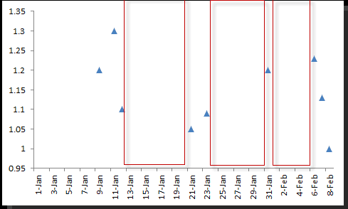
Unevenly-spaced time series are common in many real-life applications when measurements are constrained by practical conditions. The irregularity of observations can have several fundamental reasons. First, any event-driven collection process (in which observations are collected when some event occurs) is inherently irregular. Second, in such applications as sensor networks or any distributed monitoring infrastructure, data collection is distributed and collection agents can’t easily synchronize with one another. In addition, the sampling intervals and policies may be different. Finally, measurements cannot be made regularly or may have to be interrupted due to some events (either foreseen or not).
Unlike the equal-spaced time series case, intermediate observations with missing values can be safely dropped from the original series without any loss of information, and, obviously, the resultant series is unevenly spaced as well.
Many techniques have been proposed to handle time series with missing data, which in the limit can be viewed as irregularly sampled.
In data analysis practice, irregularity is a recognized data characteristic, and practitioners deal with it heuristically.
Solution 1: Convert to equally-spaced time series
- IGNORE: IGNORE the irregularity in the times and treat the data as if it were regular.
- RESAMPLE: RESAMPLE using a lower sampling rate. The reduction
simplifies the problem to one that has already been thoroughly analyzed and
for which many approaches are available.
Note: For a price time series, down-sampling requires taking the last observation in the new sample period. For this strategy’s log return, the re-sampled return is the cumulative return of all periods in the original sample periods./p>
- INTERPOLATE: Interpolate the intermediate missing values and convert the series to one with equally spaced sampling times. While this is a reasonable heuristic for dealing with missing values, the Interpolation in Excel process typically results in a significant bias (e.g. smoothing of the data) that changes the dynamics of the process, thus these models cannot be applied if the data is truly unequally spaced.
- Kernel Smoothing
- Brownian Bridging: A number of authors have suggested using continuous-time diffusion processes to find missing values. In principle, to interpolate a missing value, we assume a Brownian motion between the values immediately prior to and after the non-missing observations.
As of the date of this issue, NumXL does not support the Brownian bridging Interpolation in the Excel method.
Solution II - Use unequally-spaced time series Models
These models are slightly more complex than their equally-spaced counterpart models, and many can be viewed as an extension of the equally-spaced time series models.
Supposing $Y(t)$ is a time series with irregular sampling, we can decompose it into:
$$Y(t)=a(t)+X(t)$$
Where:
- $a(t)$ is a slowly changing deterministic function (trend component)
- $X(t)$ is a random noise component
In general, one can only observe $Y(t)$, our first goal is to estimate the deterministic component and extract the random noise$ X(t)=Y(t)-a(t)$; our second goal is to find a satisfactory probabilistic model for process $X(t)$
As of the date of this issue, NumXL does not support unevenly-spaced time series models.


