Daily Returns Analysis
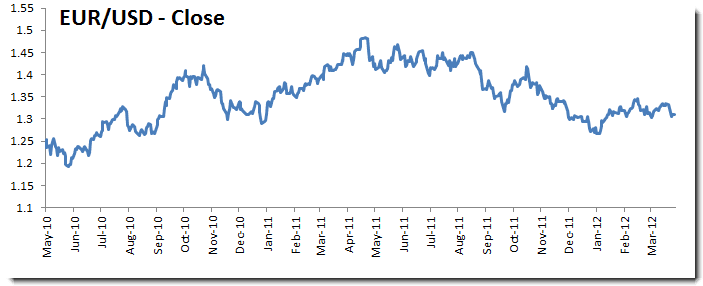
For our sample data, we use the FX exchange rate of EUR/USD between March 2010 and April 9th, 2012.
In this paper, we consider a trading strategy that buys EUR (1EUR = FX rate in USD) at market open (MOO) and closes the position (i.e. sells EUR) at market close (MOC).
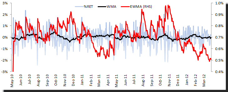
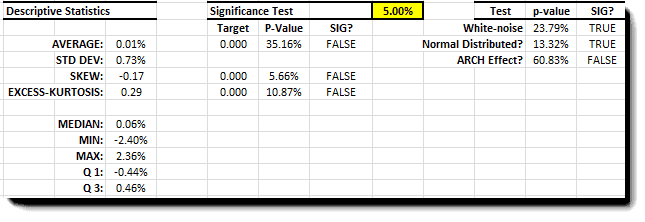
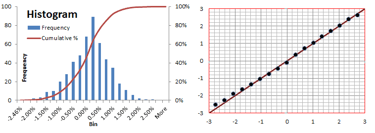
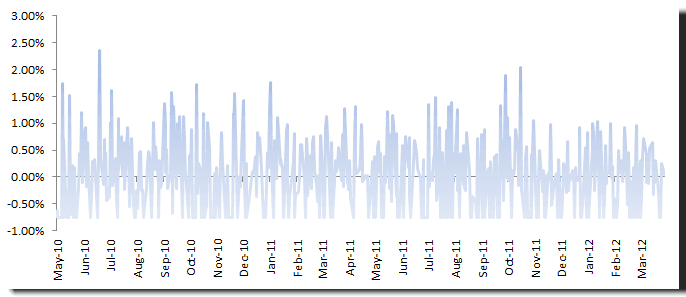
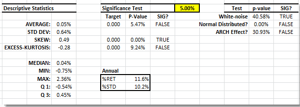
The daily returns time series shows a steady mean (proxy by 20-day WMA) and relatively stable volatility (0.5-1.0%). Examining the summary statistics, the average return is not significantly different from zero, with a symmetrical distribution and normal-like tails.
From the table on the bottom right, we can see that daily returns are more like a Gaussian distribution, and thus they possess no information.
Discussion
The daily returns act more like Gaussian noise, so the past returns do not reveal any information that can help us better predict future points. How about non-linear modeling techniques (e.g. neural networks, genetic algorithms)?
In my opinion, I would rather explore and bring new information to the analysis than spend my time utilizing sophisticated modeling techniques. In our analysis, we try to avoid the over-fitting trap and to build a robust model for reliable forecasting.
Daily High-Low time series
While we restricted our analysis to market open and close, which happen at precise times in the day, the HI and LO represent the Max-Min rates of the intra-day rates. Furthermore, they are impossible to identify for certain, so we can’t trade on them.
Nevertheless, the daily HI and LO rates bring new information that is not already in the open-close time series; as a result, we can forecast their relative levels to a certain extent.
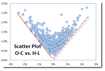
In the figure above, please note that HI-LO returns are related to the volatility of the open-close returns.
Using the sample data, we implemented a sell stop-loss order with a level set on a daily basis at the market open.
Definition: A stop loss is an order to buy or sell an asset (e.g. trading security or commodity) once the price of the asset reaches a specified price, known as the stop price. A Sell stop order is used here to limit a loss on a trading commodity we own.
Using the daily LO rate, we examine whether the stop price has breached for the day; if it breaches, we set the sale price to stop price (no slippage or transaction fees is assumed), otherwise, we continue to use the market close price for the sale price.
In this exercise, we examined the following stop price techniques: (1) Fixed percentage below the market open price (e.g. 0.75%), (2) Fixed offset below the market open price.
1. Set the stop price at a fixed percentage below the market open
Examining the summary statistics, the data exhibits positive skew and a marginally significant average.
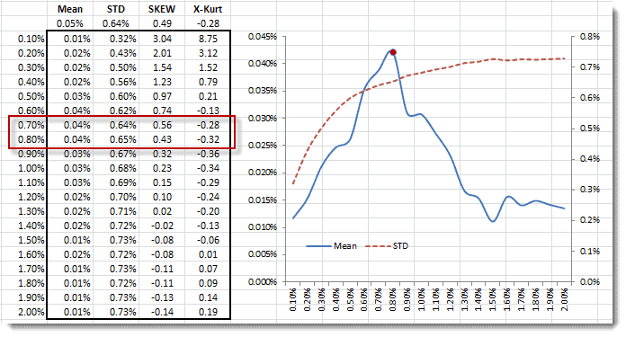
To optimize the percentage settings for the stop price, we constructed a data table where we varied the percentage between 0.1% and 2%.
Plotting the mean and volatility of the trading strategy, we picked 0.75% as the best choice. This setting gives the new trading strategy an annual return of 11.6% and a volatility of 10.2%. Furthermore, the new strategy’s returns act like white noise (but not Gaussian), so we have not left any information on the table.
2. Set the stop price as an offset below market open
In an attempt to improve the stop price strategy, we used the EWMA estimate and the WMA of the HI-LO. We followed the same steps: generate strategy returns, use a data table to examine different settings and, finally, pick the best one. The results are comparable to the simple one we illustrated above.
For detailed analysis and illustration, please refer to the Excel worksheet file (available online) for details.
Conclusion
So far, we started from a Gaussian noise data sample, incorporated daily LO rates, and devised a new strategy with stop-loss that not only limits the daily loss but generates positive returns.
Also, we can devise another strategy that employs a sell limit order to lock in profits. Using daily HI, we can examine whether the limit price is breached and construct new strategy returns.
How about a strategy that employs both: stop-loss and a limit order? Unfortunately, the data set we have doesn’t contain information about whether the HI occurs before or after the LO that day.
The takeaway here is that we can start with a data series that looks no more than Gaussian white noise. Still, with the introduction of new information (e.g., Daily HI and LO, volume, interest-rate parity, G8 summit events, etc.), we can derive a new time series with more favorable characteristics.


