Brown’s Simple Exponential Smoothing
Simple exponential smoothing is similar to the WMA except that the window size is infinite, and the weighting factors decrease exponentially.
$$Y_1=X_1$$ $$Y_2=(1-\alpha)Y_1+\alpha X_1=X_1$$ $$Y_3=(1-\alpha)Y_2+\alpha X_2=(1-\alpha)X_1+\alpha X_2$$ $$Y_4=(1-\alpha)Y_3+\alpha X_3=(1-\alpha)^2 X_1+\alpha (1-\alpha) X_2+\alpha X_3$$ $$Y_5=(1-\alpha)^3 X_1+\alpha (1-\alpha)^2 X_2+\alpha (1-\alpha) X_3 + \alpha X_4$$ $$Y_{T+1}=(1-\alpha)^T X_1+\alpha \sum_{i=1}^T (1-\alpha)^{T-i}X_{i+1}$$ $$\cdots$$ $$Y_{T+m}=Y_{T+1}$$
Where:
- $\alpha$ is the smoothing factor ($0 \prec \alpha \prec 1$)
As we have seen in the WMA, the simple exponential is suited for time series with a stable mean or a very slow-moving mean.
Example 1:
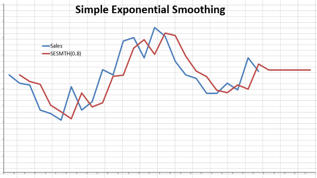
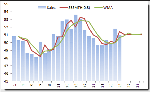
Let’s use the monthly sales data (as we did in the WMA example).
In the example above, we chose the smoothing factor to be 0.8, which begs the question: What is the best value for the smoothing factor?
Estimating the best $\alpha$ value from the data
In practice, the smoothing parameter is often chosen by a grid search of the parameter space; that is, different solutions for $\alpha$ are tried, starting with, for example, $\alpha=0.1$ to $\alpha = 0.9$, with increments of 0.1. Then $\alpha$ is chosen to produce the smallest sums of squares (or mean squares) for the residuals (i.e., observed values minus one-step-ahead forecasts; this means squared the error is also referred to as ex-post mean squared error (ex-post MSE for short).
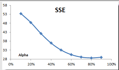
Using the TSSUB function (to compute the error), SUMSQ, and Excel data tables, we computed the sum of the squared errors (SSE) and plotted the results:
The SSE reaches its minimum value around 0.8, so we picked this value for our smoothing.
Tutorial Video
Files Examples
Please click the button below to download Brown’s Simple Exponential Smoothing example.


