Augmented Dickey-Fuller (ADF)
Over the last few months, we received many inquiries about the Augmented Dickey-Fuller (stationary test). So, we decided to create this article as a soup-to-nuts presentation on this topic.
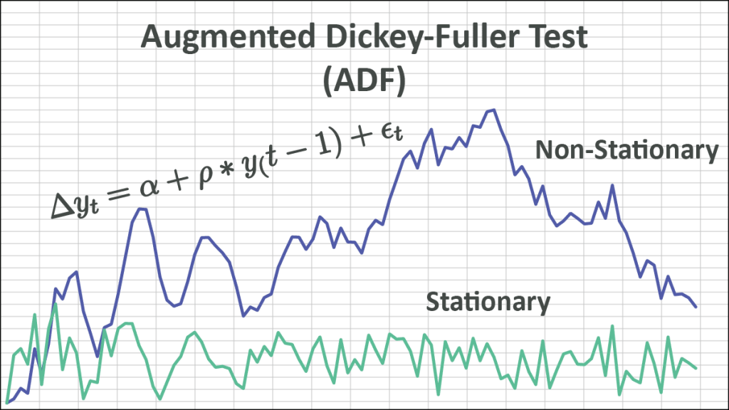
What is a stationary time series? In layman’s terms, a time series is called stationary if it does not wander off to infinity and stays around the mean. Its statistical properties (e.g., moments) do not change over time.
What about trend? Is a time series with trend considered non-stationary? Not necessarily. Time series with deterministic (i.e., non-stochastic) trend are called trend-stationary time series, but only if the time series stays around the trend-line and does not wander off to infinity.
Interesting! So how do we test whether we have a stationary (or trend-stationary) time series or not? Alternatively, we can ask a different question: what causes the non-stationary drift? A stochastic (i.e., non-stationary) drift comes from the presence of a unit-root.
To establish the stationarity assumption, we need to reject the possibility of the unit-root presence in the time series.
Where is the unit-root coming from? A non-stationary time series can be modeled as an autoregressive model (AR) of order one (1) and a coefficient value of one (1).
$$y_t=\alpha+y_{t-1}+\epsilon_t$$
Dickey-Fuller Test (DF)
In the Dickey-Fuller test, we define the underlying process as follows:
$$\Delta y_t=\alpha+\rho\times y_{t-1}+\epsilon_t$$
And set up the following test of hypothesis:
$$H_o:\rho=0$$
$$H_1=\rho<0$$
By rejecting the null-hypothesis, we are stating that the time series does not have a unit-root and is thus stationary.
Using simple-linear regression, we can compute the test-score for $\rho$, but what is the underlying distribution of $\rho$? It is not the student’s t-distribution, so we need to calculate it using simulation methods.
Simulation: For a given sample size N (e.g., 25),
- Simulate a random walk with a variance of 1:
$$y_t=y_{t-1}+ \epsilon\sim N\left(0,1\right)$$ - Run the simple-linear regression:
$$\Delta y_t=\alpha+\rho\times y_{t-1}+\epsilon_t$$ - Calculate the test score for $\rho$.
- Repeat steps 1 to 3.
Using the simulated values of the test score, construct the distribution and calculate the different critical values (e.g., 1%, 2.5%, 5%, 10%, etc.).
Using the NumXL simple linear regression (SLR) functions and the Monte-Carlo (MC) simulations Wizard, we can generate the underlying distribution by ourselves.
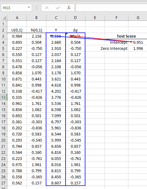
- Generate a random walk (Y) of size 25, with Gaussian shocks of variance of one (1).
- Calculate the 1st order difference of Y.
- Using the SLR functions, calculate the test score for the coefficient of the 1st parameter:
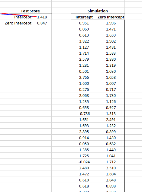
- Using the MC simulation for 1000 times, store the test-score for both regression types (zero and non-zero intercept) in empty columns.
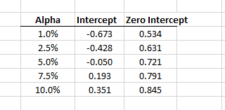
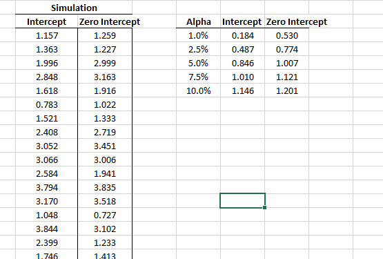
- Using the Quantile(.) function, calculate the critical values (C.V.) for different significance levels.
- Now, for a given dataset of size 25, run a similar regression and compute the test score of the coefficient value.
- Compare the regression test score against the simulation critical values.
- To establish stationarity, the test score must be smaller than the critical values (above), so we can reject the null hypothesis.
What about the trend-stationary scenario? We’d need to add a deterministic trend term in the regression:
$$\Delta y_t=\alpha+\gamma\times t+\rho\times y_{t-1}+\epsilon_t$$
To carry on the simulation, we add a constant column for the time trend and calculate the test score for Y using the multiple-linear regression (MLR) model.
Again, using the NumXL Monte-Carlo simulation, let’s generate 1000 values for the test scores and compute the test-score critical values.
Augmented Dickey-Fuller (ADF) Test
The main difference in the augmented Dickey-Fuller test is the added complexity in the regression model.
$$\Delta y_t=\alpha+\rho\times y_{t-1}+\delta_1\Delta y_{t-1}+\cdots+\delta_p\Delta y_{t-p}+\epsilon_t$$
By including lags of order p in the ADF formulation, we are allowing higher-order AR processes. This means that the lag order p must be determined when applying the test.
How do we determine the value of p? One possible approach is to start with a higher value (e.g., 5) and test down by examining the statistical significance of the coefficient (i.e., t-value).
Once we determine the optimal p and calculate the test-score of the coefficient of Y (i.e., $\rho$), we compare them against the test critical values.
The ADF test critical values can be calculated using Monte-Carlo simulations. We start with a random walk sample of a given size (e.g., 25) and calculate the test-score of the Y coefficient in the multiple linear regression model (MLR).
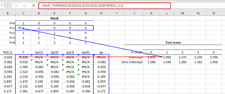
Using the NumXL MLR_PARAM(.) function, we can compute the test-score for different values of P by altering the mask argument.
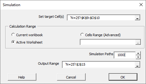
Now we are ready to run the Monte-Carlo simulation on all the MLR models.
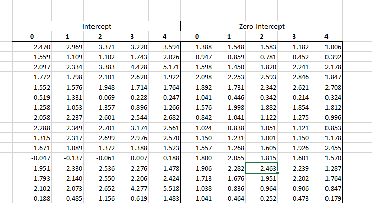
In the MC wizard, we specified the whole table as target cells. The MC wizard generates its output by scanning the target cells from left to right, then top to bottom, and writing their values in adjacent columns.
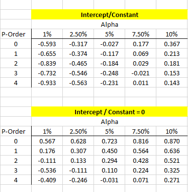
Using the simulation results, we can calculate the test critical value for N=25, different P-order values, and significance level (between 1% to 10%).
Just like we did in the original Dickey-Fuller test, to reject the null-hypothesis (presence of unit-root), we need the regression test-score of the Y coefficient to be smaller than the critical value.
What about trend-stationarity ? To examine for trend-stationarity, we need to include a trend variable in the data set, compute the test-score for the coefficient of Y, and include it in the simulation.
Conclusion
In this article, we describe the underlying assumptions for stationary tests and the mechanics for generating the test critical values for different sample sizes, significance levels, and regression models (e.g., intercept, trend) using Excel and NumXL functions.
To demonstrate the simulation technique, we ran only 1000 simulations to generate the critical values. In practice, simulations of an order of 2 million yield relatively stable critical values and are reliable for statistical testing inferences.

