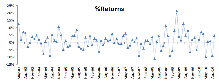
In this paper, we’ll examine a claim by a portfolio manager (let’s call him trader B) about his ability to generate statistically significant Alpha. Alpha is a risk-adjusted measure of the so-called active return on investment. In other words, Alpha is the excess-return compensation for the risk borne, and thus commonly used to assess active managers’ performances. Trader B agreed to share his monthly realized net returns (after accounting for brokerage fees and other trading expenses) between May 2003 and Sept 2010 with us to analyze.
First, we’ll look at the time series’ general statistical properties, probability distribution, QQ-Plot, and perform various statistical tests to answer some key questions.
Next, we’ll compute the excess-returns time series. For risk-free returns, we’ll use the 4-weeks T-Bill as a proxy, and re-run the same analysis we did with raw returns.
Then we’ll look closely for evidence of any outliers that may bias our analysis, which will help us identify one potential outlier in April 2009. To assess the outlier impact on our analysis, we replace its value with a plug-value and note the change on different stats.
Finally, we’ll establish a simple band to identify potential outliers that may affect our analysis and find one observation with an exceptionally high return.
In sum, the single outlier observation single-handed generates favorable results, and the returns time series does not look impressive (to say the least) without it. The question we ought to ask is, how likely is it that the outlier observation will be repeated in the future?
Analysis
For sample data, we are using an active manager portfolio’s monthly returns
between May 2003 and September 2010.
Let’s run the summary statistics of the raw monthly returns:
The monthly returns have a significant mean (i.e., no zero) and no sign of serial correlation or ARCH effect. The volatility of the strategy (5.48% per month) is similar to that of the S&P 500 index, so the time series, at first sight, indicates that it may have an alpha (aka risk-free returns).
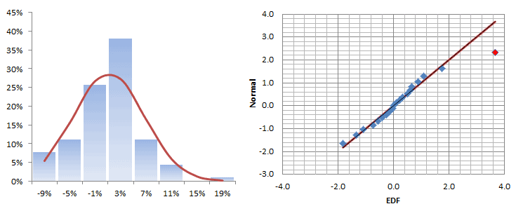
Let’s plot the distribution and QQ-Plot of those returns:
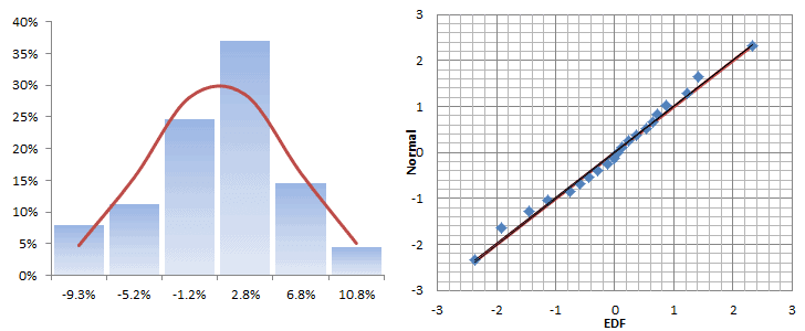
The monthly returns seem to follow a Gaussian distribution for the most part, but there is a sign of a fat tail on the right side, which is not necessarily bad, since it falls on the upside.
Now let’s redirect our focus on the excess returns:
\[ r_a = r – r_{t\to t+d}^f\]
Where
- $r_a$ is the adjusted or excess-return
- $r_f$ is the risk-free return
- $r$ is the portfolio’s raw return
For risk-free returns, we’ll use the 4-Week US Treasury bill (T-Bill) bond-equivalent yield (BEY).
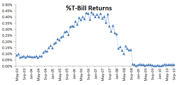
The T-Bills are issued on a weekly schedule, so we interpolate the values to align the date with the start of the holding period. To compute the bond-equivalent yield ($r_{BEY}$) of the 4-week T-Bill using the discount rate ($r_d$):
\[ r_{\textrm{BEY}}=\frac{r_d\times 365}{360-r_d\times 28} \]
Furthermore, to compute the equivalent risk-free return for a given holding period ($r_{t\to t+d}^{f}$)
\[ r_{t\to t+d}^{f}=r_{\textrm{BEY}}\times \frac{d}{365}=\frac{r_d\times d}{360-r_d\times 28} \]
Where
- $d$ is the number of days in a given holding period.
Now let’s plot the excess or the adjusted returns along with the original returns. The difference is relatively small, and we can visually distinguish the two returns apart.
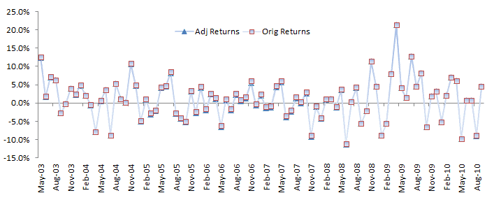
Let’s examine the general statistical properties of the adjusted returns.
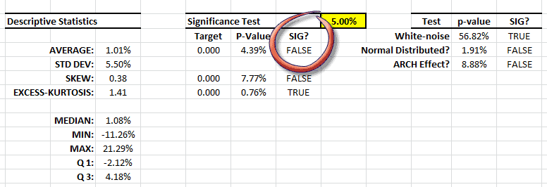
The descriptive statistics are very similar to the original data, with one exception: the population-mean is not significantly different from zero – no alpha. Interesting!
We could stop the analysis here, and refute the presence of a significant alpha – which symbolizes the portfolio manager’s skill or talent, but let’s continue and dig deeper.
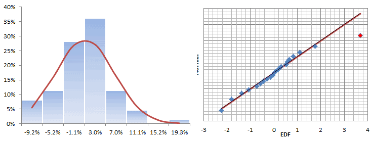
The histogram and QQ-Plot look very similar to those of the original returns, with signs of a fat tail on the right side of the distribution. There is no sign of an ARCH effect, so what is causing this fat tail?
Next, we will construct a band or contour using the inter-quartile range in an effort to identify potential outliers. Once detected, we’ll try to explain them first, and then assess their impact on our findings.
The Inter-Quartile band is described as follows:
\[ \textrm{UL}_t=\textrm{Q3}_{t_o \to t}+1.5\times \textrm{IQR}_{t_o \to t} \]
\[ \textrm{LL}_t=\textrm{Q1}_{t_o \to t}-1.5\times \textrm{IQR}_{t_o \to t} \]
In essence, we are computing the quartiles and inter-quartile range using the observation values realized to that moment.
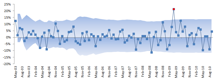
In the graph above, a few observations can pierce through the band, but only one observation stands out: In April 2009, the strategy generated 21.3% returns. This is good, right?
Whether the value is good or not is not the point here; we only care about the consistency with other observations in the sample data. Let’s assess the value’s impact on our analysis: replace the returns value for April 2009 with a plug value – say 8% (prior month return value) – and re-run the summary statistics.
The descriptive statistics table shows a Gaussian white noise distribution. The adjusted returns mean is not statistically different from zero and its volatility is ~ 17.7% per Annum. This is very similar to the S&P 500.
Conclusion
In our analysis, the original strategy returns exhibited a statistically significant mean. Some analysts may confuse this parameter with the strategy’s alpha, but they are not the same. The alpha can only be computed with excess-returns (returns beyond the risk-free investment, such as T-Bill).
Analyzing the excess-returns of the strategy, the mean is no longer significantly different from zero, but the returns distribution exhibits a fat tail on the right side. Digging deeper, we found that this is due primarily to one outlier value.
In sum, based on the provided data, the employed strategy does not yield a statistically significant alpha.
What about the returns on April 2009; should we dismiss those? It depends, but we ought to ask a different question: how likely is the returns we saw in April 2009 to re-occur in the future? If it is a one-time incident, I’d suggest dropping it from the sample data and applying a plug-value in its place.


