Interpolation 101
Many years ago, NumXL supported an interpolation function as a utility or helper method to meet our users’ modeling needs. To our surprise, this functionality received significant attention, and we decided to compile some of the most frequently asked questions about it here.
What is Interpolation?
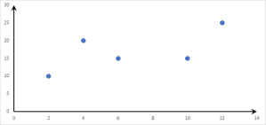
To illustrate, let’s assume the value of a function $y=f(x)$ is given as a set of five (5) distinct x-values, as shown in the plot below.
Now, we wish to estimate (i.e., interpolate) the value of the function at $x=5$, using the given five (5) data points.
For interpolation purposes, the desired target x value must be within the range of the original data set (e.g., $2\le x\le 12$).
Before we go any further, let’s answer a few foundational questions we often hear:
- What about extrapolation? How is it different? Extrapolation is the process of estimating the function value of an x-value that falls outside the range of a given dataset.
- Does NumXL support extrapolation? Yes, the same function NxINTRPL(.) can be used for extrapolation. Make sure to pass “true” or 1 to the “extrapolate” argument.
- Is curve fitting (e.g., regression) and interpolation the same? Curve fitting and interpolation are often used interchangeably, but there is a subtle difference between them: interpolation must fit the data points exactly, whereas curve fitting must get as near as possible.
- Should I use interpolation or curve fitting? It depends. Interpolation assumes that data points are known perfectly (or at least to very high precision), while curve fitting assumes some degree of noise in the data points.
Data Preparation
As we mentioned earlier, all interpolation methods accept a discrete set of known data points. To handle real-world data sets, the NumXL interpolation function (NxINTRPL) pre-processes the data to:
- Sort the data points in ascending order (based on X).
- Silently drop data points with missing values.
- Replace multiple readings for the same X value with their average.
Q: Should the data points be uniformly separated?
A: No, the interval length between data points doesn’t need to be uniform, but we recommend that datapoints are spread out over the x-range to improve the interpolation accuracy and minimize the impact of outliers.
Interpolation Methods
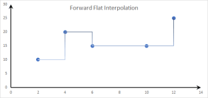
- Step Interpolation 1: Forward Flat Interpolation.
The step interpolation methods model the unknown function flat/constant between known datapoints, using the last known value.
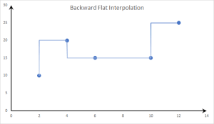
- Step Interpolation 2: Backward Flat Interpolation.
In the case of the backward flat method, the unknown function is also modeled as flat/constant between the known data points, but it uses the level of the immediate next data point.
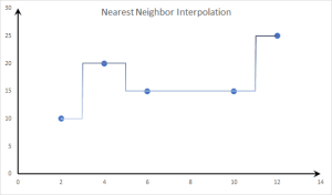
- Step Interpolation 3: Nearest Neighbor Interpolation.
With the nearest neighbor method, the unknown function is still modeled flat/constant, but its level is determined by the level of the nearest data point.
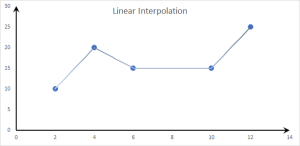
- Linear Interpolation:
With linear interpolation, we connect each data point to its neighbors using straight lines.
- Note that the values of the function between two data points is solely determined by those two data points.
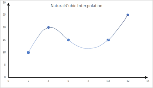
- Cubic Spline: Natural Spline
Using the cubic spline method, we construct a piece-wise cubic polynomial on each interval with matching first and second derivatives at the supplied data points. The second derivative is chosen to be zero at the first point and the last point.
- The resultant curve is smooth, but it is not “local,’ which means if the functions make a large change (e.g., x=4), the curve around the surrounding points is “wobbly” (aka., it overshoots at intermediate points).
- Cubic Spline: AKIMA Spline
To avoid the wobbly curve of the natural cubic spline, we relax the continuity of the second derivative around the data points (knots), resulting in non-rounded corners.
As shown in the figure above, the curve around the data points is continuous but not smooth.
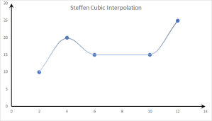
- Cubic Spline: Steffen Spline
Steffen’s spline adds a new constraint: the cubic spline segment is monotonic between data points. There is no wobbling, period.
- The resultant curve is smooth around the data points and does not exhibit any wobbling between them. Therefore, minima and maxima can only occur exactly at the data points.
- Steffen’s spline and its first derivative are guaranteed to be continuous, but the second derivative may be discontinuous.
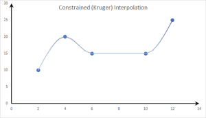
- Cubic Spline: Constrained (Kruger) Spline
Kruger proposed a constrained cubic spline to prevent overshooting by sacrificing smoothness, so we no longer require a continuous second derivative at every point and calculate the first derivative value numerically using surrounding points.
- Using the constrained (Kruger) spline, we avoided the overshoot wobbly effect of the cubic spline and did not need to add monotonicity constraints.
Q: Which type of cubic spline should I use?
A: It depends on the nature of your data, and the importance of a smooth curve and/or overshoot side-effect. In many cases, we suggest choosing the constrained (Kruger) cubic spline as a safe bet.
Q: I see two interpolation functions in NumXL: Interpolate(.) and NxINTRPL(.). Which one should I use?
A: The Interpolate(.) function was our early implementation function, but it is now deprecated. All the interpolation methods mentioned above are available only in NxINTRPL(.), so you should only use this function.
Q: The NxINTRPL(.) function accepts both a single value and an array for the target argument. Why?
A: The NxINTRPL(.) runs faster when you interpolate for multiple values at once, rather than calling separately for each value. We recommend passing all x-values in a few function calls.

