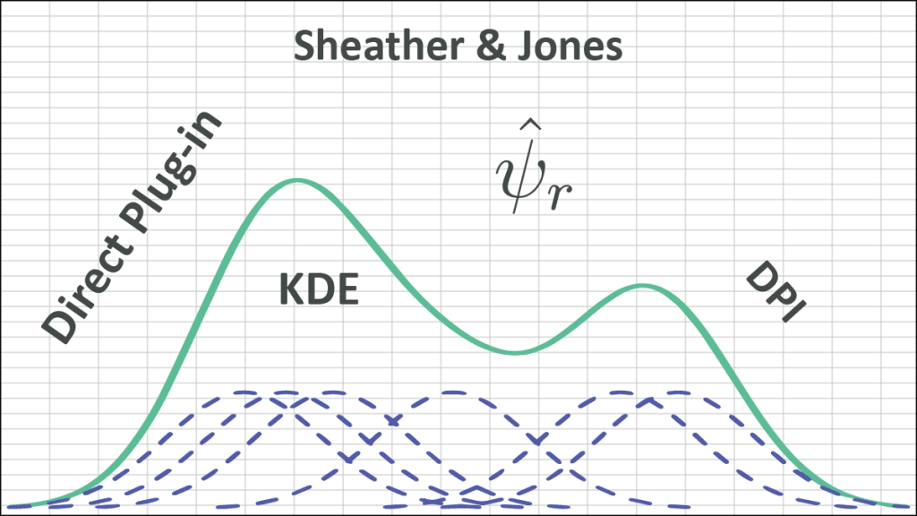
KDE – Direct Plug-In Method
A quick recap: In the KDE Optimization Primer, we derived the formula for the optimal bandwidth and the minimum AMISE, as follows:
Where:
- $R({{f}^{(2)}})$ is defined as follows:
$$R({{f}^{(2)}})=\int\limits_{-\infty }^{\infty }{[{{f}^{(2)}}(x)}{{]}^{2}}dx$$ - $R(K)$ and $\mu _{2}^{2}(K)$ are known constant quantities determined by the selection of the kernel function (e.g., Gaussian).
The main problem in using the formula above in practice is that we don’t know the value of $R({{f}^{(2)}})$: the integral of the squared second derivative of the underlying probability density function $f(x)$, which we are trying to estimate.
How can we overcome this problem? We can estimate $R({{f}^{(2)}})$ using the KDE itself.
Before we go any further, we need to introduce a neat math trick: Assuming that $\forall r>0$, the ${{f}^{(r)}}(\pm \infty )\to 0$, then the following relation holds:
So, if we are to apply it to $R({{f}^{(2)}})$:
Remember that $f(x)$ is the probability density function, so we can express $R({{f}^{(2)}})$ as follows:
In effect, we converted $R({{f}^{(2)}})$ into the expectation of the 4-th derivative of $f(x)$, which can be estimated (i.e., ${{\hat{\psi }}_{4}}$ non-parametrically using the sample data.
Where ${{\hat{f}}^{(4)}}(.)$ is a data-driven estimator of the $f(x)$ fourth derivative.
${{\psi }_{r}}$ Estimation
Using a KDE estimator with kernel function $L(.)$ and bandwidth $g$, the $\hat{f}(x;g)$is defined as follows:
$$\hat{f}(x;g)=\frac{1}{ng}\sum\limits_{i=1}^{n}{L(\frac{x-{{X}_{i}}}{g})}$$
$${{\hat{f}}^{(1)}}(x;g)=\frac{1}{n{{g}^{2}}}\sum\limits_{i=1}^{n}{{{L}^{(1)}}(\frac{x-{{X}_{i}}}{g})}$$
$$…$$
$${{\hat{f}}^{(r)}}(x;g)=\frac{1}{n{{g}^{r+1}}}\sum\limits_{i=1}^{n}{{{L}^{(r)}}(\frac{x-{{X}_{i}}}{g})}$$
Plugging in ${{\hat{f}}^{(r)}}(x;g)$, the expected r-th derivative estimator ${{\hat{\psi }}_{r}}$ is expressed as follows:
$${{\hat{\psi }}_{r}}=\frac{1}{{{n}^{2}}{{g}^{r+1}}}\sum\limits_{i=1}^{n}{\sum\limits_{j=1}^{n}{{{L}^{(r)}}(\frac{{{X}_{i}}-{{X}_{j}}}{g})}}$$
The next question is: what is $g$? It is the kernel function $L(.)$ (and the bandwidth $g$). Is it the same one we use for the final KDE? Not necessarily, as our goal is to minimize the error in the ${{\hat{\psi }}_{r}}$ estimate.
Under certain regularity assumptions (Wand and Jones (1995)), The asymptotic bias and variance of ${{\hat{\psi }}_{r}}$ are obtained, so we can compute the asymptotic mean squared error (AMSE):
And the AMSE optimal bandwidth is:
${{g}_{\text{AMSE}}}=\sqrt[r+k+1]{-\frac{k!{{L}^{(r)}}(0)}{{{\mu }_{k}}(L){{{\hat{\psi }}}_{r+k}}\times n}}$
Where:
- $k$ is the number of stages, provided ${{\mu }_{k}}(L)>0$.
- For $k=0$ (Silverman method), we start with a known distribution (e.g., Gaussian), calculate ${{\hat{\psi }}_{4}}$ (analytically), and compute the optimal bandwidth.
- For $k=2$(Direct Plug-in method), we start with known distribution (e.g., Gaussian). Then:
- Calculate ${{\hat{\psi }}_{8}}$ (analytically).
- Stage 1:
- Compute the optimal bandwidth value for estimating ${{\hat{\psi }}_{6}}$
- Calculate ${{\hat{\psi }}_{6}}$.
- Stage 2:
- Compute the optimal bandwidth value for estimating ${{\hat{\psi }}_{8}}$
- Calculate ${{\hat{\psi }}_{4}}$.
- Calculate the optimal KDE bandwidth.
- For $k=4$ (Direct Plug-in method), we start with a known distribution (e.g., Gaussian). Then:
- Calculate ${{\hat{\psi }}_{12}}$ (analytically).
- Stage 1:
- Compute the optimal bandwidth value for estimating ${{\hat{\psi }}_{10}}$.
- Calculate $ {{\hat{\psi }}_{10}}$.
- Stage 2:
- Compute the optimal bandwidth value for estimating ${{\hat{\psi }}_{8}}$.
- Calculate ${{\hat{\psi }}_{8}}$.
- Stage 3:
- Compute the optimal bandwidth value for estimating ${{\hat{\psi }}_{6}}$.
- Calculate ${{\hat{\psi }}_{6}}$.
- Stage 4:
- Compute the optimal bandwidth value for estimating ${{\hat{\psi }}_{4}}$.
- Calculate ${{\hat{\psi }}_{4}}$.
- Calculate the optimal KDE bandwidth
Typically, two stages ($k=2$) are considered a good trade-off between bias (mitigated as $k$ increases), and variance (increases with $k$).
Direct Plug-in Method (Sheather & Jones)
This is the method proposed by Sheather and Jones (1991), where they consider $L=K$ and $k=2$, yielding what we call the Direct Plug-In (DPI). The algorithm is:
- Using the sample data, calculate $\hat{\sigma }=\min (s,{{\hat{\sigma }}_{\text{IQR}}})$.
- Assume a Gaussian underlying distribution (i.e., $f(x)=\phi (x)=\frac{1}{\sqrt{2\pi }\sigma }\exp \left( -\frac{{{(x-\mu )}^{2}}}{2{{\sigma }^{2}}} \right)$), then calculate (analytically) the ${{\hat{\psi }}_{8}}$. $${{\hat{\psi }}_{8}}=\int\limits_{-\infty }^{\infty }{{{\phi }^{(8)}}(x)\phi (x)dx}=\frac{105}{32\sqrt{\pi }{{{\hat{\sigma }}}^{9}}}$$
- Calculate the optimal bandwidth for ${{\hat{\psi }}_{6}}$, ${{g}_{1}}$: $${{g}_{1}}=\sqrt[9]{-\frac{2{{K}^{(6)}}(0)}{{{\mu }_{2}}(K){{{\hat{\psi }}}_{8}}\times n}}$$
- Estimate ${{\hat{\psi }}_{6}}$: $${{\hat{\psi }}_{6}}=\frac{1}{{{n}^{2}}g_{1}^{7}}\sum\limits_{i=1}^{n}{\sum\limits_{j=1}^{n}{{{K}^{(6)}}(\frac{{{X}_{i}}-{{X}_{j}}}{{{g}_{1}}})}}$$
- Calculate the optimal bandwidth for ${{\hat{\psi }}_{4}}$, ${{g}_{2}}$: $${{g}_{2}}=\sqrt[7]{-\frac{2{{K}^{(4)}}(0)}{{{\mu }_{2}}(K){{{\hat{\psi }}}_{6}}\times n}}$$
- Estimate ${{\hat{\psi }}_{4}}$: $${{\hat{\psi }}_{4}}=\frac{1}{{{n}^{2}}g_{2}^{5}}\sum\limits_{i=1}^{n}{\sum\limits_{j=1}^{n}{{{K}^{(4)}}(\frac{{{X}_{i}}-{{X}_{j}}}{{{g}_{2}}})}}$$
- Now, using ${{\hat{\psi }}_{4}}$ as an estimate for $R({{f}^{(2)}})$: $${{h}_{\text{DPI}}}=\text{ }\sqrt[5]{\frac{R(K)}{\mu _{2}^{2}(K){{{\hat{\psi }}}_{4}}\times n}}$$
Conclusion
References
- Silverman, B.W. (1986). Density Estimation for Statistics and Data Analysis. Chapman & Hall/CRC London.
- W. Zucchini, Applied smoothing techniques, Part 1 Kernel Density Estimation., 2003.
- Byeong U. Park and J. S. Marron. Comparison of Data-Driven Bandwidth Selectors. Journal of the American Statistical Association Vol. 85, No. 409 (Mar., 1990), pp. 66-72 (7 pages).
- S.J. Sheather and M.C. Jones. A reliable data-based bandwidth selection method for kernel density estimation. J. Royal Statist. Soc. B, 53:683-690, 1991.


