Calculating Signal-to-Noise Ratio Using DFT
In an earlier issue, we presented a filtering function that uses several Fourier frequencies (hereafter referred to as components) (k) with the highest amplitude. The next question would be: what is the minimum number of components we can use that capture the vital essence (aka., information) of the original signal?
To answer this question, we introduce a new measure – used in signal processing and information theory – called the signal-to-noise ratio (SNR). The signal-to-noise ratio compares the level of the desired signal to the level of background noise.
In this issue, we will start with the trigonometric representation of the Fourier transform, calculate the average power contributed by each Fourier frequency/component (aka., power density), and estimate the signal-to-noise ratio for a generic filter function. Next, we will consider a Low-Pass Filter (LPF) – a filter that passes signals with a frequency lower than a selected cutoff frequency – and examine the change in SNR as cutoff frequency increases, and we’ll derive an approximate formula to calculate its SNR. Finally, we discuss commonly used SNR values for practical application and how we can use them to set the filter cutoff frequency.
Why Should I Care?
Compared to our previous article on Fourier Transform, this article examines the topic from a different perspective. We hope you take away, or refresh, your intuitions and reinforce these important concepts.
Background
The signal to noise ratio is defined as follows:
$$\boldsymbol{}\textrm{SNR} = \frac{P_{signal}}{P_{noise}}$$
Where:
- ${P_{signal}}$ = The average power of the desired signal.
- ${P_{noise}}$ = The average power in the background noise.
- ${\rm{SN}}{{\rm{R}}_{{\rm{dB}}}}$ = The signal to noise ratio, measured in decibels.
The background noise (N) is by definition, stochastic (indeterministic), with zero mean, so the SNR is expressed as follows:
$$SNR = \frac{{{P_{signal}}}}{{E[{N^2}]}}$$
Where:
- E[.] = the expected value operator
Note that the definition of the average power of the background noise is identical to its variance for non-deterministic (random) input signal (Q), we can express the average power as $E[{Q^2}]$.
$$SNR = \frac{{E[{Q^2}]}}{{E[{N^2}]}} = \frac{{s_Q^2 + {{\bar Q}^2}}}{{s_N^2}}$$
Because the input signal may not have a zero mean, we have ${\bar Q^2}$ in the numerator. Note that the signal-to-noise ratio is a ratio of the input and noise variances.
Discrete Fourier Transform
Given a finite sample data ${ {x_t}}$ of size N, we can express the value at time (do you mean at time t?) in terms of the corresponding discrete Fourier transform $\{ {A_i}\angle {\phi _i}\} _{i = 0}^{N – 1}$ as follows:
$$x(t) = \frac{1}{N}\left( {{A_o} + \sum\limits_{j = 1}^{N – 1} {{A_1}\cos (j \times \omega \times t + {\phi _j})} } \right)$$
$$\omega = \frac{{2\pi \times {f_s}}}{N}$$
Where:
- N = The number of observations (aka. data points) in the sample data set.
- {${A_o},{A_1},…,{A_{N – 1}}$} = the amplitudes of the DFT components.
- $\{ {\phi _1},{\phi _2},..,{\phi _{N – 1}}\}$ = the phase angles of the DFT components (measured in radians).
- ${f_s}$ = Sampling rate or frequency.
- $\omega$ = the fundamental or principle radiant frequency of the DFT.
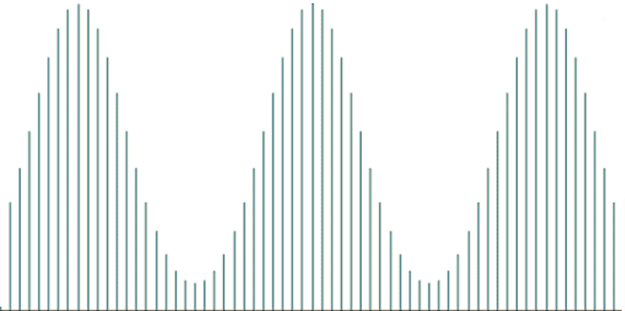
Note that DFT is symmetric around the N/2 component (or the N/2+1, if N is an even number), and repeats every N component (i.e., it is cyclical as illustrated below).
For our purposes here, and to avoid distinguishing between odd and even-sized sample data, we use the full spectrum $\{ 0,1,2,.., N – 1\}$ in our derivation below.
Why do we use DFT here?
The cosine functions in the expression above are orthogonal (uncorrelated) with each other, so calculating the mean and variance for the signal expressed as the weighted sum of those cosine functions are greatly simplified.
Let’s compute the mean of the signal:
Now, let’s subtract the mean from the values of the data points:
$$x(t) – \bar X = \frac{1}{N}\sum\limits_{j = 1}^{N – 1} {{A_1}\cos (j \times \omega \times t + {\phi _j})} $$
The variance of the input signal (${s^2}$) is defined as follows:
Let’s expand this expression:
And, the $s^2$ can be expressed as follow:
In sum, the variance of the input signal can be expressed as follow:
$${s^2} = \frac{1}{{2{N^2}}} \times \sum\limits_{j = 1}^{N – 1} {A_j^2}$$
Therefore, every DFT component contributes $\frac{{{A^2}}}{{2{N^2}}}$ to the signal variance (or power).
Filter Function
For any given a filter function, we have two signals: Input $\{ {I_t}\}$ and the filtered output signal (${O_t}$).
The background noise is simply the difference between the two signals:
$$\{ {N_t}\} = \{ {O_t} – {I_t}\}$$
The Discrete Fourier Transform (DFT) for input and filtered output signals are: $ {A_i}\angle {\phi _i}\} _{i = 0}^{N – 1}$ and $\{ {B_i}\angle {\theta _i}\} _{i = 0}^{N – 1}$, respectively, and the DFT of the noise signal (${C_i}\angle {\gamma _i}\} _{i = 0}^{N – 1}$) is also the difference between the DFT of the two signals.
$${C_i}\angle {\gamma _i} = {A_i}\angle {\phi _i} – {B_i}\angle {\theta _i}$$
Note that calculation of ${C_i}\angle \gamma$ involves complex numbers, which requires both the real and imaginary parts to be subtracted.
Let’s examine a simple filter function, where it does not affect the phase angle of the frequency component, just the amplitude, then ${\gamma _i} = {\phi _i} = {\theta _i}$ and ${C_i} = ({A_i} – {B_i})\angle {\phi _i}$
Voila! We can calculate the SNR solely using the amplitudes of the DFT of the input and output signal.
From now on, let’s consider an odd-sized sample (N). Using the symmetry property of DFT, we can use only the 1st half of the spectrum, and the SNR can be expressed as follows:
Low-Pass Filter
For a low-pass filter (LPF) function, as the cutoff frequency increases, the SNR ratio also increases; as it permits more frequency components to pass through.
For LPF(K), the output DFT is expressed as follows:
$${B_j} = \left\{ {\begin{array}{*{20}{c}}
{\begin{array}{*{20}{c}}
{{A_j}}&{j < K}
\end{array}}\\
{\begin{array}{*{20}{c}}
0&{j \ge K}
\end{array}}
\end{array}} \right.$$
The SNR is further simplified:
$$SNR(K) = \frac{{A_o^2 + \sum\limits_{j = 1}^{K – 1} {A_j^2} }}{{\sum\limits_{j = K}^{N/2} {A_j^2} }}$$
Let’s examine the marginal change when one more frequency component (say, K-component) is permitted to pass throughout the filter:
As we increase the value of the filter cutoff frequency (i.e., K), the numerator approaches 1.0 rapidly; thus, we can approximate the SNR formula as follows:
$${\rm{SNR(K + 1)}} \approx \frac{{{\rm{SNR(K)}}}}{{1 – A_K^2/\sum\limits_{j = K}^{N/2} {A_j^2} }}$$
$$\frac{{{\rm{SNR(K + 1)}}}}{{{\rm{SNR(K)}}}} \approx 1 + \frac{{A_K^2}}{{\sum\limits_{j = K + 1}^{N/2} {A_j^2} }}$$
Using the formula, we can calculate the SNR:
$$SNR(1) = \frac{{A_o^2}}{{\sum\limits_{j = 1}^{N/2} {A_j^2} }}$$
$$SNR(2) = SNR(1) \times \left( {1 + \frac{{A_1^2}}{{\sum\limits_{j = 2}^{N/2} {A_j^2} }}} \right)$$
$$SNR(3) = SNR(2) \times \left( {1 + \frac{{A_2^2}}{{\sum\limits_{j = 3}^{N/2} {A_j^2} }}} \right)$$
$$SNR(M) = SNR(M – 1) \times \left( {1 + \frac{{A_{M – 1}^2}}{{\sum\limits_{j = M}^{N/2} {A_j^2} }}} \right)$$
LPF Cutoff Frequency
Before we can address the LPF cutoff frequency issue, we need to decide on a target SNR. What is a good SNR target value? For a start, any value greater than one (or ${\rm{dB}} > 0$) indicates that there is more signal power than the background noise.
For best results, we’d seek an SNR value of 32 (i.e.,${\rm{dB}} \ge 15$) or more.
Now, we can identify a minimum cutoff frequency that yields an SNR value closest to 32.
Conclusion
In this article, we used the low-pass filter function to demonstrate the calculation of the signal-to-noise ratio between the output (filtered) signal and the input signal. We assumed any difference between the two signals is simply background noise. Furthermore, we claimed no knowledge of the original signal, but instead, used the output filtered signal as a proxy.
You can apply the same principles used in this article but to different filter functions. The formulas may differ slightly, but the rationale remains the same.


