Backtesting in Excel
Backtesting in modeling refers to a predictive model’s testing using historical data. The article is about how to do so in Microsoft Excel, not about the theoretical background of backtesting.
How do we conduct backtesting? We rewind the time to the beginning of our time series, calibrate the subject-model parameters using available data up to that instance of time, and conduct a prediction (i.e., forecast) for the next period. Next, we advance the time, recalibrate the parameters’ values and perform another projection, and so on. At the end of our exercise, we’d have a set of predictions.
Note that at each point, the only assumption we make is the general model definition (e.g., ARMA(1,1)). Still, we’d calibrate the parameters’ values using only the information available up to that instance of time.
This approach is consistent with real-life practices: first, we start with an initial model and conduct a forecast for the following period. Time moves on. A new period occurred, so we append the new data-point to the current input data set, recalibrate the parameters, conduct a forecast for the following period, and repeat.
Why should I care?
This article will take you through the steps in Microsoft Excel needed to conduct backtesting We will mainly use two powerful excel built-in functions: INDEX(.) and SEQUENCE(.), and leverage Excel’s “Data table” mechanism to run the different scenarios.
The backtesting generates what would-have-been forecasting errors, so you can closely examine the prediction error time series for serial correlation, distributions, outliers, and others, to better understand the model’s accuracy and performance.
Let’s dig in!
For this issue, we are using a synthetic stationary data set of 200 observations. The data set follows an ARMA(1,1) process, as shown next.
The proposed model is ARMA(1,1)
Backtesting Procedure
For every iteration, we need to do the following: (1) define the input data set (as sub-set of the original time series), (2) using the data set in (1), calibrate the parameters’ values of the ARMA(1,1) model, (3) Using the model in (2) and the dataset in (1), calculate a forecast for one-period ahead.
1. Input data set
To fully describe the input data set, we require two indices: start and finish, then, using the SEQUENCE(.) function, we generate a set of indices between the start and finish. Now, we use the INDEX(.) function to return all cell-range in the original data set with row-indices in the sequence set.
Example:
The original input data set is $A$3:$A$202. To select the cells between indices 1 and 50.
=INDEX($A$3:$A$202,SEQUENCE(50,1,1,1),1
Note that you can define a name for your input data and reference this name in place of the input cell range.
2. Calibrate the Model
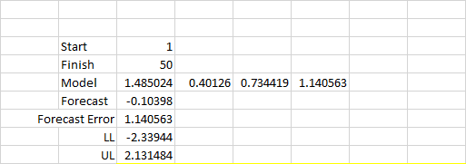
We will use the NumXL ARMA_PARAM(.) function and specify return type=2 for calibrated parameters.
Note that ARMA_PARAM(.) returns a compact form of the model’s parameters, so in the figure above, the ARMA process is: \[\begin{array}{l} {X_t} = 1.485 + 0.401{X_{t – 1}} + 0.734{a_{t – 1}} + {a_t}\\ {a_t} \sim N(0,1.14) \end{array}\]
3. Forecasting
Using the ARMA_FORE(.), data set in (1), and the model parameters calculated in 2, we can calculate the forecast values for the 1-period ahead.
Note that I generated the mean forecast, forecast error, and confidence interval.
Data Table
Now, we have just completed the calculation of one step. We will use Excel’s “Data table” feature to do the same math for the remaining periods up to step 200.
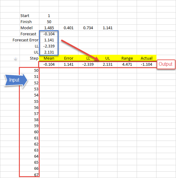
First, we need to prepare the output table:
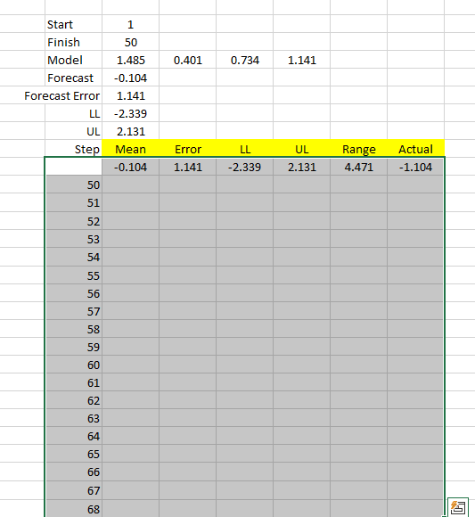
Now, select the whole data table, starting with the output row and including the finish index column, as shown below:
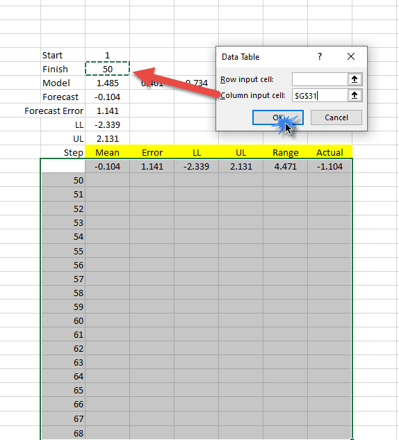
Next, switch to the “Data” Toolbar and locate the “Data Table” item under “What-if Scenario.”
The “Data Table” dialog pops up. Locate the “column input cell,” enter a reference to the “finish” index of the data set, and click the OK button.
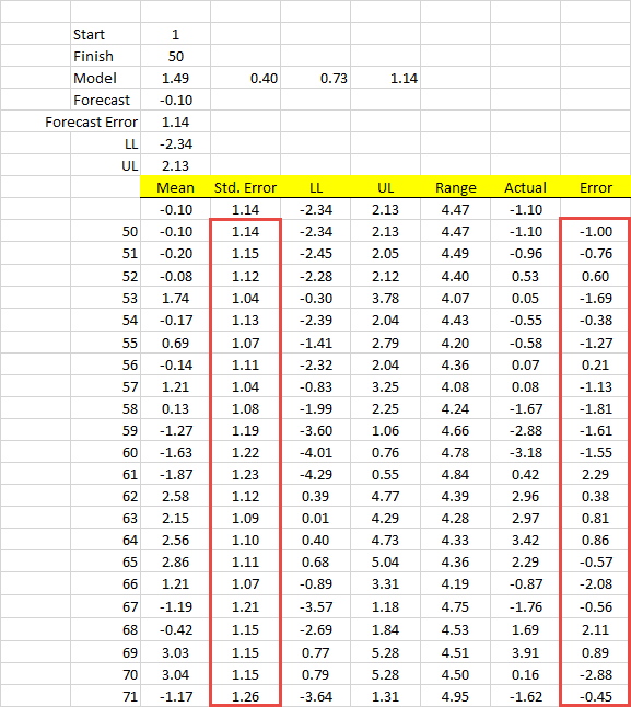
The data table will substitute the finish index’s value with the ones in our data table and store the outputs.
Note that “Std. Error” is generated by the ARMA_FORE(.) function, while the right-most column (“Error”) is the error between forecast and actual realized value.
Back-Testing Analysis
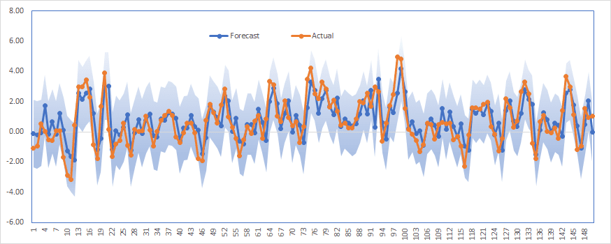
First, Let’s examine the backtesting forecast outputs visually to actual realized values, and then we will delve deeper into the statistical properties.
The shaded area in the plot corresponds to the 95% forecast confidence interval.
The plot exhibits a good model fit and, thus, forecast accuracy.
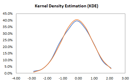
Next, let’s examine the forecast error (Forecast – Actual) statistical properties using summary statistics in the NumXL toolbar.
In conclusion, the ARMA(1,1) is a suitable predictive model for the given data set.
What is next?
By now, you are probably wondering about the values of the model’s parameters? Are they stable?
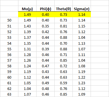
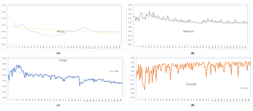
First, we construct a second “Data Table,” but in the output row are the model parameters’ values, and run the data table just like we did earlier.
Now, analyze the values of every parameter as we did with the forecast error.
The values of the parameters (except theta) exhibit stability and a trend toward a constant value. The theta (MA coefficient) values are more volatile but bound between 0.6 and 0.9.
Next, we should examine the descriptive statistics and the underlying distributions of the parameters’ values, but we will leave this exercise to you.
Conclusion
This article demonstrated the steps to conduct backtesting for a predictive model with minimal or no intermediate calculation. We have used Excel’s built-in functions: INDEX(.) and SEQUENCE(.) and leveraged the “Data Table” feature to run the calculation for all pre-defined indices.
Once we had the backtesting results, we turn our heads to statistical analysis and evaluate their properties and distribution to uncover any biases (e.g., serial correlation) in the output.
Files Examples
Please click the button below to download Back-testing example.


