Hurst Exponent in Excel
Occasionally, our support desk receives inquiries about Hurst exponent: what is it? How do we use it in Excel? And how do we interpret the calculated values? In this issue, we will go over the Hurst exponent in-depth, and hopefully, help you develop an intuition and insight for the Hurst exponent.
What is Hurst exponent?
The name “Hurst exponent“, “Hurst Index“, or “Hurst coefficient“, derives from Harold Edwin Hurst (1880–1978), who was the lead researcher in these studies. Studies involving the Hurst exponent were initially developed in hydrology for the practical matter of determining optimum dam sizing for the Nile river’s volatile rain and drought conditions that had been observed over a long period.
The Hurst exponent (H) is used as a measure of long-term memory of time series. It relates to the time series’s autocorrelations and the rate at which these decrease as the lag between pairs of values increases. The Hurst exponent is often referred to as the “index of dependence” or “index of long-range dependence.”
What Is The Long Memory Of A Process?
Long memory, also called Long-range dependence (LRD) or long-range persistence, is a phenomenon that may arise in time-series data. It relates to the decay rate of statistical dependence of two points as the time between the points increases.
Does the ARMA (P, Q) process exhibit a long memory?
No! A stationary ARMA with finite P and Q orders, ARMA(P, Q), has a short memory. You can examine the autocorrelation function (ACF) plot as its value decays exponentially and dies out after a few lags.
How does a long-memory model behave?
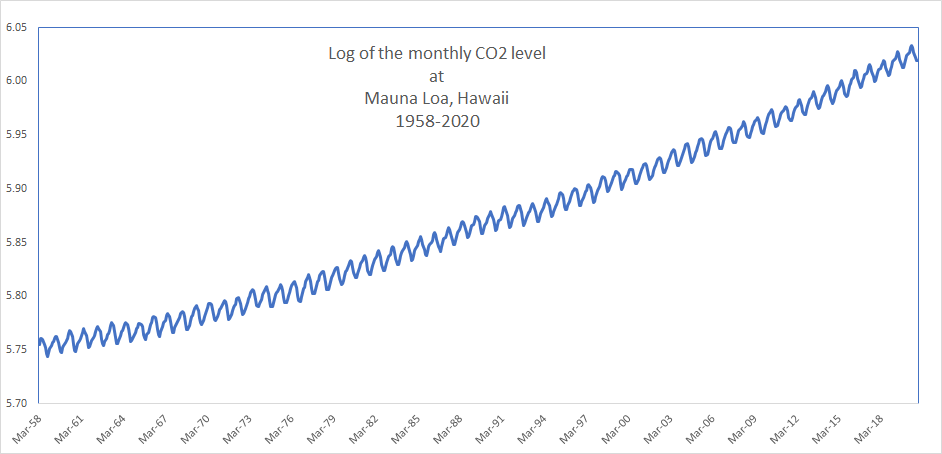
In general, a process with a long memory may look like a slow random-walk (drifting), with a slow decaying autocorrelation function. For example, let’s examine the monthly average carbon dioxide (CO2) level recorded in Mauna Loa, Hawaii weather station.
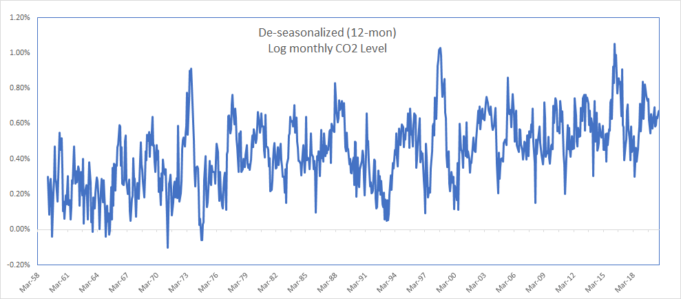
Next, let’s remove the 12-month seasonality by differencing the value of each observation, from one that is 12-month earlier.
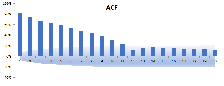
In the correlogram plot, the autocorrelation factors (ACF) are decaying, but at a very slow pace.
How do we model the long-memory time series?
Just like we did in the non-stationary ARIMA model: we extract the fractional integration component and capture the short-memory in the residuals with an ARMA model. Using fractional difference operator, we capture the long-memory dynamic in a time series:
\[{(1 – L)^d} = \sum\limits_{k = 0}^\infty {\left( {\begin{array}{*{20}{c}} d\\ k \end{array}} \right)} {( – 1)^k}{L^k} = 1 + {\omega _1}L + {\omega _2}{L^2} + …\]
Where:
- $L$ = Lag or Backshift operator
- ${\omega _1} = – d$
- ${\omega _2} = – \frac{{{\omega _1} \times (d – 1)}}{2}$
- ${\omega _N} = – \frac{{{\omega _{N – 1}} \times (d – N – 1)}}{N}$
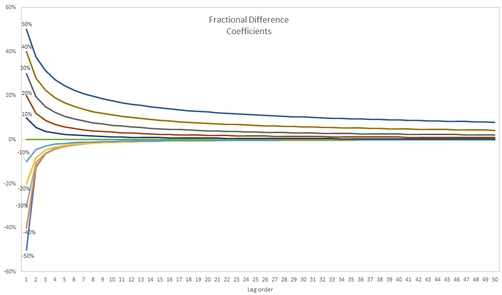
For $\left| d \right| \le \frac{1}{2}$, the coefficient ${\omega _k}$ decay power-like relatively quickly (yet, slower than the exponential decay).
Putting it all together, we end up with fractional ARIMA (i.e., FARIMA)
\[(1 – {\phi _1}L – {\phi _2}{L^2} – … – {\phi _p}{L^p}){(1 – L)^d}{X_t} = (1 + {\theta _1}L + {\theta _2}{L^2} + … + {\theta _q}{L^q}){a_t}\]
Where:
- $L$ = Lag or Backshift operator
- ${X_t}$ = time series data set
- ${a_t}$ = innovation (or shocks) time series
- $d$ = integration order, and its value between -0.5 and 0.5, exclusive.
How do we find out the integration order (d)?
The fractional integration order (d) is equal to the Hurst exponent (H) minus 0.5 (i.e, d = H – 0.5)
Interpretation
In a nutshell, the Hurst exponent is a single value (H), which we can use to draw an observation about the time series long-memory (serial correlation):
| H | Interpretation |
|---|---|
| 0.5 - 1.0 | a time series with long-term positive autocorrelation. |
| 0.0 - 0.5 | indicates a time series with long-term switching between high and low values in adjacent pairs, meaning that a low value will probably follow a single high value and that the value after that will tend to be high, with this tendency to switch between high and low values lasting a long time into the future. |
| 0.5 | a completely uncorrelated series, but in fact, it is the value applicable to series for which the autocorrelations at small-time lags can be positive or negative but where the absolute values of the autocorrelations decay exponentially quickly to zero. |
Hurst Exponent Calculation in Excel
Let’s go over how to calculate Hurst Exponent in Excel. The original and best-known method for estimating the Hurst exponent is the so-called rescaled range (R/S) analysis based on Hurst’s previous hydrological findings.
The NumXL Hurst(.) function calculates the original (empirical) Hurst exponent when you set the return type = 1.
=Hurst(x, Alpha,1)
However, this approach is known to produce biased estimates. For a small sample size, there is a significant deviation from the 0.5 slopes (i.e., uncorrelated long-range).
Size-Corrected (Anis-Llyod) Estimate
To correct the built-in bias in the original (empirical) Hurst exponent estimate, Anis-LIyod introduced a size-corrected estimate of the rescaled range (R/S).
The NumXL Hurst(.) function calculates the Anis-Llyod (corrected R/S) Hurst
exponent when you set the return type = 2.
=Hurst (X,Alpha,2)
Statistical Significance
No asymptotic distribution theory has been derived for most of the Hurst exponent estimators so far. However, we have an approximate functional form for the confidence intervals of the Anis-Lloyd corrected R/S analysis.
To examine the statistical significance of the calculated Hurst exponent estimate(), we construct the following test of the hypothesis:
\[\begin{array}{l} {{\rm{H}}_o}:{H_q} = {\rm{ uncorrelated}}\\ {{\rm{H}}_1}:{H_q} = {\rm{ long – memory}} \end{array}\]
Next, we calculate the corresponding Hurst exponent estimate and the confidence interval (C.I.) limits of an uncorrelated (no long-memory) time-series for a given sample size.
The NumXL Hurst(.) function calculates the Anis-Llyod (corrected R/S) Hurst
exponent for uncorrelated time-series of the same size when you set the return
type to 3.
=Hurst(X, Alpha,3)
NumXL Hurst(.) function calculates the lower and upper limits of the confidence
interval of Anis-Llyod Hurst exponent of the uncorrelated time-series when you
set the return type to 4 and 5, respectively.
					LL=Hurst(X,Alpha,4)
UL=Hurst(X, Alpha,5)
Finally, we examine the Anis-Llyod (corrected R/S) Hurst exponent value against the C.I. of the Null-hypothesis (uncorrelated time series).
- The Hurst exponent estimate is outside the C.I.; thereby, the time series has a long memory.
- The Hurst exponent is inside the C.I., thereby, the time series does not exhibit a significant long memory property, and observations can be uncorrelated.
Hurst Exponent Analysis In Excel
Let’s examine the 12-month deseasonalized log CO2 level between March 1958 and November 2020.
The Anis-Llyod corrected R/S Hurst exponent estimate is 0.84, and this value is outside the C.I. of Hurst exponent of an uncorrelated time series of the same size. The de-seasonaled CO2 log level time series exhibits a long-memory behavior, and the fractional difference order (d) is 0.34 (i.e., 0.84 -0.50 = 0.34).

