Kernel Density Estimation (KDE) Plot
Previously, we’ve seen how to use the histogram method to infer the probability density function (PDF) of a random variable (population) using a finite data sample. In this tutorial, we’ll carry on the problem of probability density function inference, but using another method: Kernel density estimation.
Kernel density estimates (KDE) are closely related to histograms but can be endowed with properties such as smoothness or continuity by using a suitable kernel.
Why do we care?
One of the main problems in practical applications is that the needed probability distribution is usually not readily available, but rather it must be derived from other existing information (e.g. sample data). KDEs are similar to histograms in terms of being a non-parametric method, so there are no restrictive assumptions about the shape of the density function, but KDE is far superior to histograms as far as accuracy and continuity.
Overview
Let’s consider a finite data sample $\{x_1,x_2, \cdots ,x_N\}$ observed from a stochastic (i.e. continuous and random) process. We wish to infer the population probability density function.
In the histogram method, we select the left bound of the histogram $(x_o )$, the
bin’s width (h ), and then compute the bin k probability estimator $f_h(k)$:
- Bin k represents the following interval $[x_o+(k-1)h, x_o+k\times h)$
- $\hat f_h(k)$ is defined as follow: $$\hat f_h(k) =\frac{\sum_{i=1}^N I\{(k-1)h\leq x_i-x_o\leq k\times h)\}}{N}$$
- $I\{.\}$is an event function that returns 1 (one) if the condition is true, 0 (zero) otherwise.
The choice of bins, especially the bin width (h ), has a substantial effect on the shape and other properties of $f_h(k)$.
Finally, we can think of the histogram method as follows:
- Each observation (event) is statistically independent of all others, and its occurrence probability is equal to $\frac{1}{N}$.
- $f_h(k)$ is simply the integral (sum) of the event probabilities in each bin.
What is a kernel?
A kernel is a non-negative, real-valued, integrable function $K(.)$ satisfying the following two requirements:
$$\int_{-\infty}^{\infty}K(u)du=1$$ $$K(u)=k(-u)$$
$$K(u)=k(-u)$$
And, as a result, the scaled function $K^*(u)$, where $K^*(u)=\lambda K(\lambda \times u)$, is a kernel as well.
Now, place a scaled kernel function at each observation in the sample and compute the new probability estimators $f_h(x)$ for a value x (compared to an earlier bin in the histogram).
$$\hat f_h(x)=\frac{1}{N}\sum_{i=1}^N K_h(x-x_i)$$
$$K_h(u)=\frac{1}{h}K(u/h)$$
$$\hat f_h(x)=\frac{1}{N\times h}\sum_{i=1}^N K((x-x_i)/h)$$
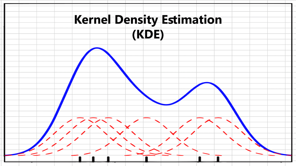
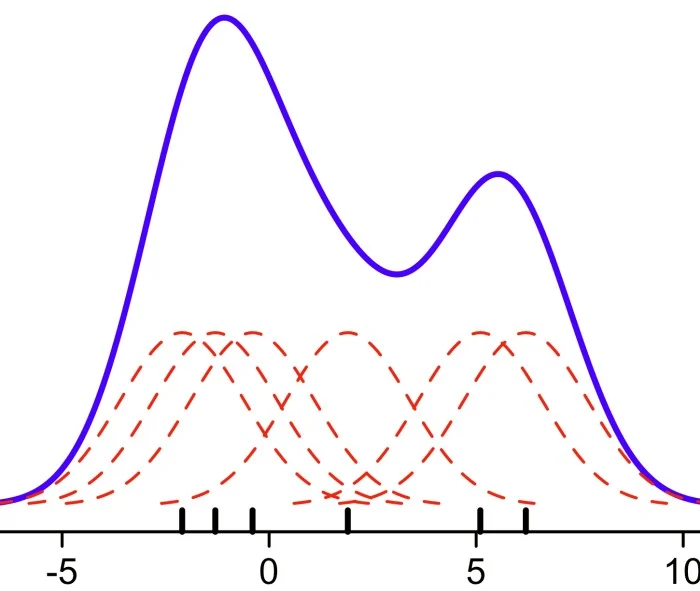
As an example, let $K(.)$ be the standardized Gaussian density function. The KDE looks like the sum of Gaussian curves, each centered on one observation.
Note: For the Gaussian kernel, the bandwidth is the same as the standard deviation of ($x-x_i$ ).
The KDE method replaces the discrete probability:
$$P(x)=\left\{\begin{matrix} \frac{1}{N} & x \in \{x_1,x_2,\cdots , x_N\} \\ 0 & x \notin \{x_1,x_2,\cdots , x_N\} \end{matrix}\right.$$
With a kernel function. This permits overlap between kernels, thus promoting
continuity in the probability estimator.
Why KDE?
Due to our data sampling, we are left with a finite set of values for continuous random variables. Using a kernel instead of discrete probabilities, we promote the continuity nature in the underlying random variable.
To proceed with KDE, you’ll need to decide on two key parameters: Kernel function and bandwidth.
Which kernel should I use?
A range of kernel functions is commonly used: uniform, triangular, biweight, triweight, and Epanechnikov. The Gaussian kernel is often used; $K(.)=\phi(.)$, where $\phi$ is the standard normal density function.
How do I properly compute kernel bandwidth?
Intuitively, one wants to choose an h value as small as the data allows, but there is a trade-off between the bias of the estimator and its variance.
The selection of the bandwidth of a kernel estimator is a subject of considerable research. We will outline two popular methods:
- Subjective selection – One can experiment by using different bandwidths and simply selecting one that “looks right” for the type of data under investigation.
- Selection with reference to some given distribution – Here one selects the
bandwidth that would be optimal for a particular PDF. Keep in mind that you
are not assuming that $f(x)$ is normal, but rather selecting an h which would be optimal if the PDF were normal. Using a Gaussian kernel, the
optimal bandwidth $h_{opt}$ is defined as follows:
$$h_{opt}=\sigma\times \sqrt[5]{\frac{4}{3N}}$$
The normal distribution is not a “wiggly” distribution; it is uni-modal and bell-shaped. It is therefore to be expected that $h_{opt}$ will be too large for multimodal distributions. Furthermore, the sample variance ($s^2$ ) is not a robust estimator of $\sigma^2$; it overestimates if some outliers (extreme observations) are present. To overcome these problems, Silverman proposed the following bandwidth estimator:
$$h_{opt}=\frac{0.9\times \hat\sigma}{\sqrt[5]N}$$
$$\hat \sigma = \textrm{min}(s,\frac{R}{1.34})$$
$$R=IQR=Q3-Q1$$
Where $IQR$ is the interquartile range and “$s$” is the sample standard deviation. - Data-driven estimation – this is an area of current research using several different methods: Fourier transform, diffusion-based, etc.
Conclusion
In this tutorial, we demonstrated the process to generate a kernel density estimation in Excel using NumXL’s add-in functions.
The KDE method is a major improvement for inferring the probability density function of the population, in terms of accuracy and continuity of the function. Nevertheless, it introduces a new challenge: selecting a proper bandwidth. In the majority of cases, the Silverman estimator for the bandwidth proves to be satisfactory, but is it optimal? Do we care?
Where do we go from here?
First, to answer the question of optimality, we need to introduce additional algorithms to estimate its values. For example, in “Annals of Statistics, Volume 38, Number 5, pages 2916-2957”, Z. I. Botev, J. F. Grotowski, and D. P. Kroese described a numerical sample data-driven method for finding the optimal bandwidth using a Kernel density estimation via the diffusion approach.
Second, in cases where the range of values that the random number can take are known to be constrained from one side (e.g. prices, binomial data, etc.), or in a range (e.g. survival rate, default rate, etc.), then how do we adapt the KDE to factor in those constraints?
Finally, we defined the KDE probability estimator using a fixed bandwidth ( ) for all observations. If the bandwidth is not held fixed but is varied depending upon the location of either the estimate (balloon estimator) or the samples (pointwise estimator), this produces a particularly powerful method known as adaptive or variable bandwidth kernel density estimation.
Files Examples
Please click the button below to download Kernel Density Estimation (KDE) example.


