Principal Component Analysis (PCA) 102
This is the second entry in our principal components analysis (PCA) in Excel series. In this tutorial, we will resume our discussion on dimension reduction using a subset of the principal components with a minimal loss of information. We will use NumXL and Excel to carry out our analysis, closely examining the different output elements in an attempt to develop a solid understanding of PCA, which will pave the way to more advanced treatment in future issues.
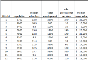
In this tutorial, we will continue to use the socioeconomic data provided by Harman (1976). The five variables represent the total population (“Population”), median school years (“School”), total employment (“Employment”), miscellaneous professional services (“Services”), and median house value (“House Value”). Each observation represents one of twelve census tracts in the Los Angeles Standard Metropolitan Statistical Area.
Process
Now we are ready to conduct our principal component analysis in Excel. First, select an empty cell in your worksheet where you wish the output to be generated, then locate and click on the principal component (PCA)icon in the NumXL tab (or toolbar).
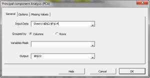
The Regression Wizard will appear.
Select the cells to range for the five input variable values.
- The cell range includes (optional) the heading (Label) cell, which would be used in the output tables where it references those variables.
- The input variables (i.e., X) are already grouped in columns (each column represents a variable), so we don’t need to change that.
- Leave the “Variables Mask” field blank for now. We will revisit this field in later entries.
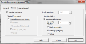
Next, select the “Options” tab.
Initially, the tab is set to the following values:
- “Standardize Inputs” is checked. Leave this option checked.
- “Principal Component Output” is checked. Uncheck it.
- The significance level (aka. α�) is set to 5%.
- “Input Variables” is unchecked. Check this option.
- Set “No. of PCs included” to 3. This action can be done now or altered later in the output tables, as our formulas are dynamic.
- Under “Input Variables”, check the “Values” option, so the generated output tables include a fitted value for the input variables using a reduced set of components.
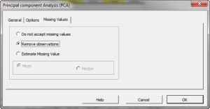
Now, click the “Missing Values” tab.
In this tab, you can select an approach to handle missing values in the data set (X and Y). By default, any missing value found in any observation would exclude the observation from the analysis.
This treatment is a good approach for our analysis, so let’s leave it unchanged.
Now, click “OK” to generate the output tables.
Analysis
1. Statistics
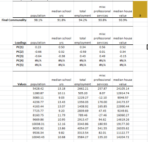
In this table, we show the percentage of the variance of each input variable accounted for (a.k.a final communality) using the first three (3) factors. Unlike the cumulative proportion, this statistic is related to one input variable at a time.
Using this table, we can detect which input variables are poorly presented (i.e., adversely affected) by our dimension reduction. In this example, the “median school years” has the lowest value, yet the final communality is still around 92%.
2. Loadings
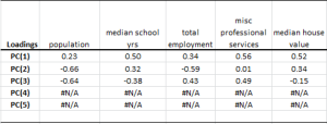
In the loading table, we outline the weights of the principal component in each input variable:
To compute the values of an input variable using PC values, we use the weights above to linearly transform them back. For example, the population factor is expressed as follows:
$$\hat X_1=0.23PC_1-0.66PC_2-0.64PC_3$$
- This table is basically the transposed table (rows turned into columns) that we saw in the variables’ loadings for PCs.
- The sum of the squares of each row must be 1.
- $PC_1,PC_2,PC_3,\cdots, PC_m$ are are uncorrelated, so to compute the
variance of $X_1$(Standardized),using the first k-components:
$$Var(\hat X_i)=\gamma_1^2\sigma_1^2+\gamma_2^2\sigma_2^2+\cdots+\gamma_k^2\sigma_k^2 \leq 1$$ $$X_i=\frac{x_i-\bar x_i}{\sigma_{x_i}}$$ $$\gamma_1^2\sigma_1^2+\gamma_2^2\sigma_2^2+\cdots+\gamma_m^2\sigma_m^2=1$$ Where:- $\gamma_k$ is the loading of the k-th principal component for the $X_i$ input variable.
- $\sigma_k^2$ is the variance of the k-th principal component.
- $X_i$ is the estimate for the standardized input variable using the first k-components.
- By definition, the $Var[\hat X_i]$ is the final communality.
- The variance of the fitted input variable in the original scale (non-standardized)
is expressed as follows:
$$Var[ \hat{x_i} ]=(\gamma_1^2\sigma_1^2+\gamma_2^2\sigma_2^2+\cdots+\gamma_k^2\sigma_k^2)\times \sigma_{x_i}^2$$ - Reducing the dimension, in essence, reduces the variance of the input variables (low pass filter).
- What about the correlation among original variables? How are they affected
by reducing the dimensions?
$$\hat X_i=\gamma_1PC_1+\gamma_2PC_2+\cdots+\gamma_kPC_k$$ $$\hat X_j=\omega_iPC_1+\omega_2PC_2+\cdots+\omega_kPC_k$$ $$Cov[\hat X_i, \hat X_j]=\sigma_{\hat X_i,\hat X_j}=E[\hat X_i \times \hat X_j]=E[\gamma_1\omega_1PC_1^2+\gamma_2\omega_2PC_2^2+\cdots+\gamma_k\omega_kPC_k^2 ]$$ $$Cov[\hat X_i, \hat X_j]=\rho_{\hat x_i,\hat x_j}= \sum_{i=1}^k \gamma_i\omega_i\sigma_i^2$$ $$Cov[X_i, X_j]=\rho_{x_i,x_j}= \sum_{i=1}^m \gamma_i\omega_i\sigma_i^2=\sigma_{\hat X_i,\hat X_j}+\sum_{i=k+1}^m \gamma_i\omega_i\sigma_i^2$$ $$Cov[\hat X_i, \hat X_j] = Cov[X_i, X_j] - \sum_{i=k+1}^m \gamma_i\omega_i\sigma_i^2$$ Where:- $\hat X_i$ is the standardized fitted i-th variable using the first k-principal components.
- $X_i$ is the original standardized i-th input variable.
- $x_i$ is the original i-th input variable.
- $\hat x_i$ is the non-standardized fitted i-th input variable using the first k-principal component.
- How about covariance between the variables (non-standardized)? $$\hat X_i = \frac{\hat x_i-\bar x_i}{\sigma_{x_i}}\Rightarrow \hat x_i-\bar x_i=\hat X_i \times \sigma_{x_i}$$ $$Cov[\hat x_i,\hat x_j]=E[(\hat x_i-\bar x_i)(\hat x_j-\bar x_j)]=\sigma_{x_i}\sigma_{x_j}E[\hat X_i\hat X_j]$$ $$Cov[\hat x_i,\hat x_j]=\sigma_{x_i}\sigma_{x_j}\times (\sigma_{X_i,X_j}-\sum_{i=k+1}^m \gamma_i\omega_i\sigma_i^2)$$ $$Cov[\hat x_i,\hat x_j]=Cov[x_i,x_j]-\sigma_{x_i}\sigma_{x_j}\sum_{i=k+1}^m \gamma_i\omega_i\sigma_i^2$$
In sum, the relative change in covariance is equal to the change in correlation between the two variables.
Note: Reducing the number of factors alters the statistical characteristics of the underlying data set, so extreme care must be taken.
3. Fitted Values
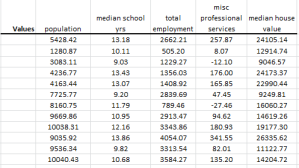
Using the first three (3) principal components, NumXL calculates the fitted value for each input variable:
Although the principal components analysis in Excel uses the standardized version of the input variables, it computes the fitted values in the original non-standardized format.
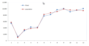
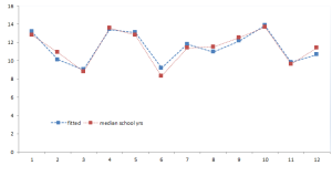
Let’s plot the population (highest final communality) and median school years (lowest final communality) for the original data and for the fitted one.
Conclusion
In this tutorial, we examined the dimension reduction proposition from 5 PCs to 3 PCs without significant loss of information.
What do we do now?
In the first two tutorials, we focused on delivering the key ideas behind the principal component analysis and, to some extent, the rationale behind the dimension reduction proposition. The cross-section socio-economic sample data, although not a time series, served to demonstrate the theory and to show NumXL’s different output tables.
In the third entry of this series, we are ready to look into a set of correlated time series and apply the PCA technique to derive a reduced core set of uncorrelated drivers. Next, we forecast the values (mean and standard error) for the uncorrelated drivers and using the PCA Loadings, imply the corresponding forecast (mean and error) for each input variable.

